
Before making a costly Flash purchase, it’s always a good idea to use some science to forecast if the new storage hardware configuration, and especially the costly Flash you purchase, is going to be able to handle your workload. Is your planned purchase performance capacity actually too much, so that you aren’t getting your money’s worth? Or, even worse, is your planned hardware purchase too little?
In Part 1 of this blog, we discovered that our customer just might be planning to purchase more Flash capacity than their unique workload requires. In part 2 we will demonstrate how we were able to use modeling techniques to further understand how the proposed new storage configuration will handle their current workload. We will also project how this workload will affect response times when the workload increases into the future, as workloads tend to do.
Step 1: Stress the Box
When we model a workload on a storage system, we want to select a workload that, first, represents the real customer workload. And second, the model should represent that workload during peak periods. We normally select two peak periods, one during high I/Os per second (IOPS) and the other during high throughput (MB/sec). We break the workload down into many different performance components and select the interval that puts the most stress on the different parts of the storage system we are modeling.
These storage system parts include the internal bus, storage controllers, disk drives, the controllers handling the I/O to the host systems, and many others. Later we will refer to the load on many of these components. As for the unique workload components we look at, Figure 1 shows a snapshot of one of our worksheets for the max. IOPS selection. We had a month’s worth of data – about 3000 lines on the spreadsheet. From that we selected the top 10 IOPS intervals, and looked for the intervals that would apply the most stress.
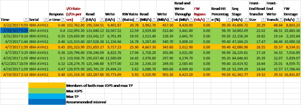
Figure 1: I/O Metrics
Figure 2 shows this interval on the throughput graphs.
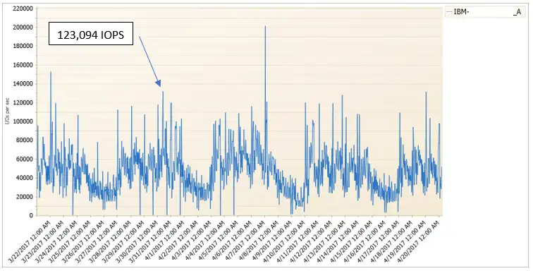
Figure 2: Throughput
Step 2: Configure the Model
After selecting the time interval we want to model, it’s time to configure our models. We have one model for each time interval. Our modeling software is IntelliMagic Direction. Most of you have probably heard of IBM’s modeling software, Disk Magic – that’s our product. IntelliMagic Direction is just our version of that modeling software. Figure 3 shows the first page of the modeling software. This is where we input the details of the proposed hardware configuration and the Easy Tier settings from Part 1 of this blog. Notice the tabs across the top. The interfaces tab is where we detail the disk controllers and the host interfaces. The disk tab is for the disk configuration.
And the Workload tab, shown in Figure 4, is where we input the details from the IOPS workload we selected in Step 1, above.
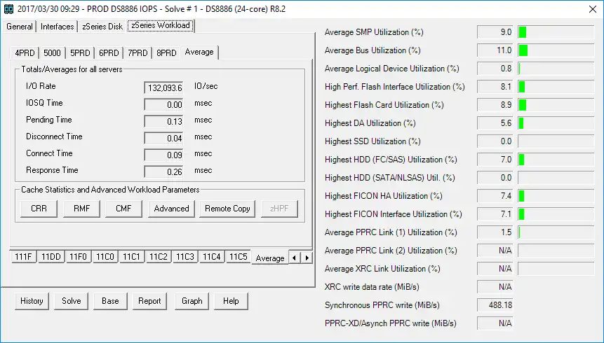
Figure 4: zSeries Workload
Once the model is populated with data, we hit the Solve button on the bottom. After this step, we see the utilizations the workload imposes on the different hardware components of the storage system, shown in the right-hand pane. I referred to these hardware components in Step 1, above.
Step 3: Understand the Results
There’s a bunch of different ways to look at the results of the model. The one we use often for these types of studies is the utilization overview shown in Figure 5. This shows all the different storage system hardware components and their utilizations as the model increases the workload.
Proposed Configuration
The first data point is 132,094 IOPS, which was our peak interval for throughput. The model then increases that workload until something breaks. In this case, the last interval is 1,032,094 IOPS where the device adaptors that control the spinning disk drives just can’t take anymore. Notice the disk drives themselves, the processor complex and the internal bus are not far behind. The first warning that things are becoming stressed is at 832,094 IOPS which represents a 530% increase in workload. Assuming the workload increases 3% per month, this storage system can sustain the increasing workload for over 5 years before it hits an early warning (amber) threshold, and over 5½ years before it hits the exception (red) threshold at 1,032,094 IOPS.
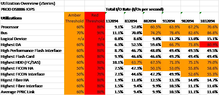
Figure 5: Utilization overview (proposed configuration)
Another modeling result we always look at is how response times increase as the workload increases. Figure 6 shows how response times go from 0.28ms to 0.5ms (yellow) to just under 0.8ms (red).
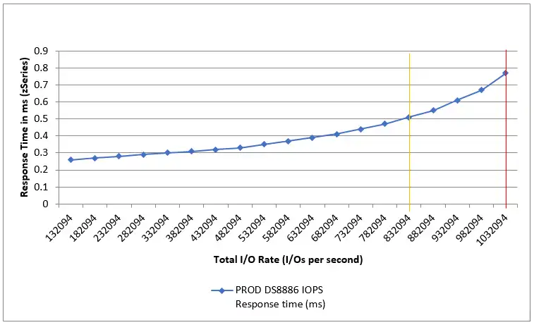
Figure 6: Response time (proposed configuration)
Half Flash Configuration
Before we get too deep into the weeds with modeling results, let’s bring this discussion back around to answering the question of how much Flash do I need?
We ran this throughput model with two different hardware configurations. The first one was the proposed hardware configuration our customer was originally planning to purchase. The second hardware configuration we considered was with half that amount of Flash. Those results are shown below in Figure 7 and 8.
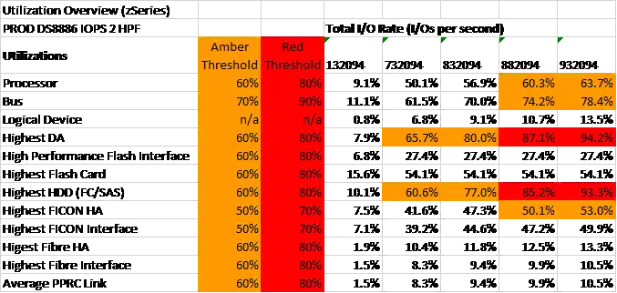
Figure 7: Utilization overview (half Flash)
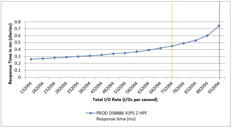
Figure 8: Response time (half Flash)
As you can see, the results with half the Flash show a modest decrease before we hit the first warning threshold of 732,094 IOPS. At the same 3% monthly I/O growth rate, the first warning threshold will be reached in 4.8 years. The first exception (red) threshold is at 882,094 IOPS which will take 5.3 years to reach. Also, the response times are virtually the same.
Our discussion so far has been using the peak I/O rate interval which normally imposes the higher stress on the Flash because they contain the greatest chance for small random I/Os. We also went through this exact same exercise with the peak throughput (MB/sec) interval. It is important for the modeling of both the peak IOPS and peak throughput to pass the test before we can conclude that the half-Flash configuration will handle the workload.
Summary: Proving the Configuration
Our models using IntelliMagic Direction confirmed our findings in Part 1 of the blog and allowed the customer to save a lot of money. We could determine how long their proposed hardware configuration would stand up against their current workload at a conservative growth rate of 3% and last for the length of a typical storage system.
If you have any questions about our findings or the calculations that were done, or if you would like to model your own future configuration, send us an email at info@intellimagic.com.
This article's author
 Jim Sedgwick
 Share this blog
Related Resources
Should I Disable SVC Write Cache for Flash?
It has been suggested that in order to maximize throughput for large sequential operations on SVC volumes residing entirely on IBM Flash systems, you should consider disabling the write cache.
How Much Flash Do I Need? Part 1
Flash has many benefits, but it's still costly. This blog demonstrates how it is possible to determine how much Flash is important to add, and how much would be a wasted spend.
How’s Your Flash Doing?
Since most storage management algorithms optimize their enterprise storage automatically, you may not have the time or tools to quantify how your Flash is performing.
Book a Demo or Connect With an Expert
Discuss your technical or sales-related questions with our mainframe experts today