
Sub-Capacity MLC Pricing
With the recent IBM announcement about Tailored Fit Pricing, it seems an opportune time to discuss the current pricing methods, to help decide if the new option is the right ‘fit’ for your datacenter.
In this first blog I’ll cover sub-capacity pricing, followed by capping, and will conclude with a blog devoted to the new tailored fit pricing model. Each of these methods comes with its own set of pros and cons, and as with most things, which one is best for your datacenter depends on a lot of different factors.
Sub-Capacity Pricing Background
In decades past, software billing was based on the full capacity of the machine(s). Several years ago, IBM introduced sub-capacity pricing, allowing installations to only pay based on their ‘average peak’ consumption. The term ‘average peak’ seems contradictory, so allow me to elaborate.
The Rolling Four-Hour Average (R4HA) is a calculated value based on system utilization in Millions of Service Units (MSU). (R4HA is also commonly referred to as 4HRA or 4-Hour Rolling Average. They both refer to the same thing, but for the purposes of this blog I will use R4HA.) Each IBM machine has an MSU rating. This is very much like MIPS as it is a measure of capacity. This capacity is consumed by the LPARs and applications on the machine on an on-demand basis.
As application consumption is based on, often unpredictable, demand, CPU/MSU may be very high or low at any moment in time. To allow for these brief spikes in consumption, IBM calculates the R4HA every five minutes.
Each hour, the system takes the average of these 12 five-minute values. After four hours, the system will then have a true “Four-Hour Average”. As time goes on, the calculation continues to “roll” so you then have a continuously updated Rolling Four-Hour Average (R4HA). This is the ‘average’ part.
Each month, via the SCRT report (technically this is from midnight (the very beginning) of the second day of the month up to midnight (the very beginning) of the second day of the next month) the peak R4HA hour is reported and this is the basis for the software bill. This is the ‘peak’ part.
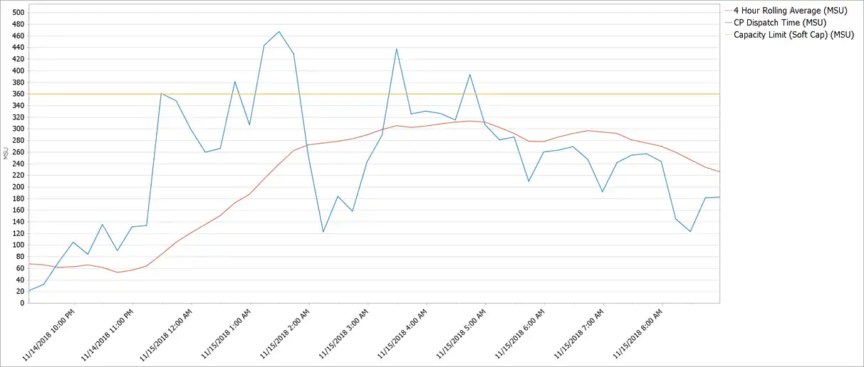
The following IntelliMagic Vision chart illustrates a common area of confusion. One peak drives capacity; the other drives costs.
 LPAR Scope
 LPAR Scope
Note that the R4HA (SMF70LAC) has an LPAR scope and is stored in the SMF 70 record. Quite often, it is necessary to calculate a R4HA for multiple LPARs. In this case they are added together.
Note that the peak value is not the “sum of the peaks” but rather the “peak of the sums”. That is to say, the hour with the highest combined peak of the combined LPARs, not necessarily the highest peak of any individual LPAR or sub-group.
Subsystem Billing
Most subsystems (IBM software products) such as z/OS, DB2, CICS, IMS, etc. are billed on individual rates per subsystem. While products are licensed on a CPC/CEC basis, the installation has the option to start or not start a product on a given LPAR. Products are only billed on an LPAR if they are started. This is an easy way to avoid unnecessary MLC charges. Note that once a product is started on a given LPAR – even for a moment – it will be billed for that billing cycle. SCRT tracks this via the SMF 89 record.
One further note on subsystem billing: the invoice is based on total MSU consumption on the LPAR(s) where a given subsystem is started; not what the subsystem is actually consuming. Every MSU of consumption contributes to the bill whether or not the subsystem is actually utilized.
In other words, if you have IMS started on a given LPAR and the workload is entirely batch jobs that never use IMS, all of the MSU consumption generated by those batch jobs contributes to the IMS bill.
LPARs and Subsystem scope
Combining the previous two points is how billing is actually calculated. The peak R4HA for every LPAR that hosts a given subsystem on a CPC is combined to calculate the invoice for that subsystem. If CICS, for example, is started on two LPARs on the CPC then the combined R4HA for those two LPARs will determine the invoice for CICS. If z/OS is running on all LPARs on the CPC (as is common) then the entire machine R4HA determines the z/OS bill. These peak hours may be on completely different days in the month. SCRT will report all this.
Standard Workload License Charges (CEC/CPC scope)
Sub-capacity pricing rates are organized into tiers. The first few MSU’s are very expensive and the incremental rate decreases as the capacity increases. With standard WLC this is done within CEC/CPC boundaries.
Consider the above example, where CICS is running on two LPARs. Assume, for this example that CICS is running on two LPARs on each CEC/CPC. The combined R4HA peak of each of the two LPARs on each machine will be calculated separately. On each machine, they start at zero MSU and measure up through the WLC tiers. The two values are then added together to determine the CICS invoice.
Country Multiplex Pricing (CMP)
CMP (also known as Country Wide Multiplex) is an offering from IBM that allows installations with more than one CEC/CPC to take advantage of workload distribution without cost penalties. As discussed above, the traditional WLC model utilizes a CEC/CPC scope.
CMP allows MSU’s billed to subsystems to cross machine boundaries provided all the machines are within the same geographical country. Consider once again, the CICS example from above. Under CMP, the MSU’s from the four CICS LPARs (two on each machine) would be added together and the total determines the tier (incremental rate) which is very likely lower.
CMP Baseline (‘the catch’)
When an installation switches to CMP, IBM requires that you provide the last three months of SCRT reports. They will average this consumption to determine a ‘baseline’ for CMP billing. In short, if your consumption does not change under CMP your bill will not change.
The primary benefit of CMP is that future growth will be at a lower incremental rate. If your consumption is decreasing, you may even pay more by moving to CMP. Assuming this is not the case (your business is growing) your best course of action is to lower your MSU consumption as much as possible in the three months prior to converting to CMP.
Next up, Capping
So far, I’ve discussed how sub-capacity pricing works and what affects your monthly IBM bill. In the next blog, “Controlling MLC with Capping,” I’ll cover capping 101 topics
How to Use Processor Cache Optimization to Reduce z Systems Costs
Optimizing processor cache can significantly reduce CPU consumption, and thus z Systems software costs, for your workload on modern z Systems processors. This paper shows how you can identify areas for improvement and measure the results, using data from SMF 113 records.
This article's author
 John Baker
 Share this blog
Related Resources
Why Am I Still Seeing zIIP Eligible Work?
zIIP-eligible CPU consumption that overflows onto general purpose CPs (GCPs) – known as “zIIP crossover” - is a key focal point for software cost savings. However, despite your meticulous efforts, it is possible that zIIP crossover work is still consuming GCP cycles unnecessarily.
Top ‘IntelliMagic zAcademy’ Webinars of 2023
View the top rated mainframe performance webinars of 2023 covering insights on the z16, overcoming skills gap challenges, understanding z/OS configuration, and more!
Mainframe Software Cost Savings Playbook
Learn how to effectively reduce mainframe costs and discover strategies for tracking IBM software licensing metrics to minimize expenses.
Book a Demo or Connect With an Expert
Discuss your technical or sales-related questions with our mainframe experts today