
The focus of this blog is on Physical Sequential datasets. As the name implies, Physical Sequential datasets are usually accessed sequentially. These are datasets defined with DSORG=PS. The concept of Physical Sequential datasets is unique to z/OS and is one of the big advantages of z/OS architecture because it enables the system to ensure that the disk space for sequential data is contiguous on the physical disk storage.
Ensuring that the data is contiguous enables the DSS hardware to do efficient prestaging and to do sequential detection. But, in order to help ensure that the dataset is entirely contiguous, z/OS uniquely has the concept of dataset extents.
Traditionally the user specifies a primary extent quantity in order to reserve some contiguous space. Secondary extents may also be allocated, although the extents may not be next to each other. If the volume is SMS-managed, DFSMS will try to allocate secondary extents contiguously if it can.
BSAM vs. SAM
Most I/O to Physical Sequential datasets is done by the BSAM access method. Some I/O is done by QSAM. BSAM is used by most high-level languages like COBOL and PL/I. Db2 and DFP Utilities also use BSAM. The ISPF editor uses BSAM.
Unlike QSAM, BSAM users manage their own buffers and have a great deal of influence on the performance. Once upon a time, when buffers were constrained by 24-bit virtual storage, applications were stingy about allocating lots of buffers. When 31-bit storage began to be used, the compilers and other applications began to use more buffers, but ISPF did not. The ISPF editor continues to use a single buffer. Likewise, IEBGENER is a very inefficient DFP Utility for copying a dataset; ICEGENER is much better.
QSAM tends to be used more by assembler programs that do not want to take the trouble of managing logical records. QSAM does an adequate job of performance, but users can do better by specifying a large value for BUFNO on their JCL.
What is Good I/O Response Time?
I/O performance analysts typically use I/O response time to evaluate performance and they have some preconceived notions of what a good or bad response time is.
For example, these days a good I/O response time for a 4KB cache hit in the DSS is around 200 to 300 microseconds, depending on the speed of the channel and DSS host adapter. I/O analysts also look at the response time components, which include connect time and disconnect time. Disconnect time is expected for cache misses. Disconnect time can be reduced by using Solid State Disks.
But what are the expectations for sequential I/O? If the DSS can prestage the data into the cache, there will be no disconnect time even if the data must be read from disk.
On the other hand, if the application reads 128KB, 256KB or 512KB per I/O, performance will be much better because there are fewer I/Os. And yet, the larger the data transfer quantity is, the higher the average connect time. In other words, in this case, high connect time is goodness.
Let’s consider an example that the device is capable of reading at a rate of 400 MB/sec. Now let’s say that the application needs to read 4GB of data. How many seconds should this take? The answer is 10 seconds. If the application reads 400KB per I/O, then it will need 10,000 I/Os to read 4GB. If the I/Os are done serially non-stop, then the average I/O response time is 1 millisecond, or 1000 microseconds. This is not an unreasonable expectation today, without any disconnect time.
Understanding Good Block Size (BLKSIZE parameter)
Another relevant performance factor for Physical Sequential datasets is the block size, or BLKSIZE parameter.
Users used to code BLKSIZE on their JCL or on ISPF menu 3.2. Some still do, not knowing what a good block size is. A good block size for a Physical Sequential dataset is half-track, which is 27998 bytes on a 3390 volume. If the user omits BLKSIZE, the system will determine the block size. So, block size issues are rare these days, but programmers do make mistakes. SMF 42 helps to find those mistakes.
A good block size for a Physical Sequential dataset is half-track, which is 27998 bytes on a 3390 volume.
If RECFM=FB (Fixed Length Blocks), then BLKSIZE must be a multiple of LRECL, the logical record size. LRECL doesn’t matter to Db2 when it uses BSAM for image copy datasets, but Db2 needs the block size to be a multiple of 4096 bytes. Thus, Db2 always chooses BLKSIZE=24576 for image copies on Disk. Image copies won’t perform quite as well as datasets that use a larger block size, but BLKSIZE=24576 is much better than BLKSIZE=4096.
So, when we look at the overall response time of a volume and observe a response time of 1 millisecond, is that good? Not if the I/Os are random 4K reads and the device type is Solid State Disk. Yes, if the I/O is sequential and the disconnect time is small. But, at a volume level, there are many datasets and applications that all use the same volume. In order to decide the goodness of an I/O response time, we need SMF 42 records.
System Managed Storage and Extended Format
It is useful at this point to review some of the objectives of System Managed Storage.
One of the objectives was to give the Storage Administrator more control over the allocation of Disk storage. With System Managed Storage, datasets must be cataloged; this helps to ensure that there are no orphaned datasets. With System Managed Storage, the administrator can implement policies through the use of 4 SMS constructs called Storage Group, Storage Class, Management Class and Data Class. The administrator codes an ACS (Automatic Class Selection) for each SMS construct.
A dataset is SMS-managed if and only if it has an SMS Storage Class assigned to it. An important parameter is called Guaranteed Space. DFSMS will automatically choose a volume for dataset allocation within a Storage Group, and if Guaranteed Space is NO, then the user cannot choose his own volume. The Storage Administrator can also specify striping requirements via Storage Class and the user cannot override this requirement if Guaranteed Space is NO.
The main purpose of Data Class is JCL simplification. All of the JCL dataset parameters can be specified as part of the Data Class definition, including the SPACE parameter. Thus, by assigning a Data Class, the administrator can control the amount of space used. Data Class may also be used to specify the DSNTYPE parameter.
Extended Format (EF) is a type of dataset (DSNTYPE) that was introduced for System Managed Storage. Non-EF datasets became known as DSNTYPE=BASIC. EF datasets require system managed storage. EF datasets use a fixed block architecture, even when RECFM=VB. I/O to EF datasets can only be done by Media Manager. Therefore, EXCP cannot be used and IMS/OSAM cannot use them. Since not all applications can use them, not all Physical Sequential datasets can use Extended Format. But Extended Format is required for the following functions:
- Increase the number of extents per dataset to 123 extents per volume
- Increase the total number of extents per dataset to 255
- QSAM buffer management improvements
- Striping
- Compression
- Encryption
VSAM is beyond the scope of this blog, but VSAM datasets can also have Extended Format. Only the functions and the performance characteristics are somewhat different.
DFSMS Compression
Extended Format datasets—both VSAM and non-VSAM datasets—can be compressed by the access method, but compression works differently in each case. SAM, which is the I/O Driver for both BSAM and QSAM, does block-level compression. VSAM can only do record-level compression. Also, because VSAM uses record-level compression, it cannot use the zEDC hardware for compression. The same is true of Db2.
Collectively BSAM and QSAM are known simply as SAM. SAM always does block level compression, because SAM is always used for sequential processing. SAM supports three different compression algorithms (and all of them are block-level):
- Generic
- Tailored
- zEDC
Generic compression uses a generic compression dictionary that is supplied with z/OS. A tailored dictionary is derived when a dataset is allocated as DISP=OLD. Tailored compression is better than generic compression for large datasets. The dictionary is based on a sample of some number of bytes and then stored at the beginning of the data set before SAM begins to write data. (Db2 also builds a tailored dictionary in the same way, but Db2 does row level compression in order to support random access. VSAM, on the other hand, always uses generic compression.)
zEDC (z Enterprise Data Compression) is the newest type of compression, introduced in z/OS 2.1. EDC compression for new datasets can be requested in a similar manner to how the existing types of compression (generic or tailored compression) are requested. It can be selected at the system level, the Data Class level, or both.
Figure 1 contains the data set information for a compressed data set that uses zEDC as shown by IntelliMagic Vision for z/OS.
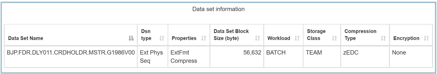
Figure 1: Data set information
The Dsn type column indicates “Ext Phys Seq” and the Properties column indicates “ExtFmt Compress”. The Compression Type column indicates zEDC. Here the block size of 56,632 bytes is the physical block size, not BLKSIZE value. The Storage Class name is also shown here. The WLM Workload name is also shown as a dataset characteristic. If two different jobs belong to different workloads use the same dataset, two rows will appear in the table showing different Workload names.
Figure 2 illustrates a report generated by IntelliMagic Vision showing the top 30 datasets ranked by Compressed Read Throughput for a 4-hour batch window, when a lot of Physical Sequential datasets tend to be read.
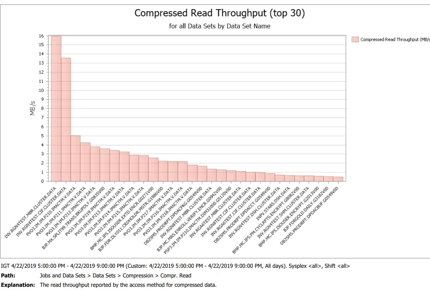
Figure 2: Compression read throughput
Figure 3 illustrates a By Time drilldown for INV.RGN4TEST.MBR.CLUSTER which is the dataset with the highest compressed read throughput. This is a VSAM dataset, but the report looks the same for any dataset type. Notice that the peak throughput exceeded 90 MB/sec.
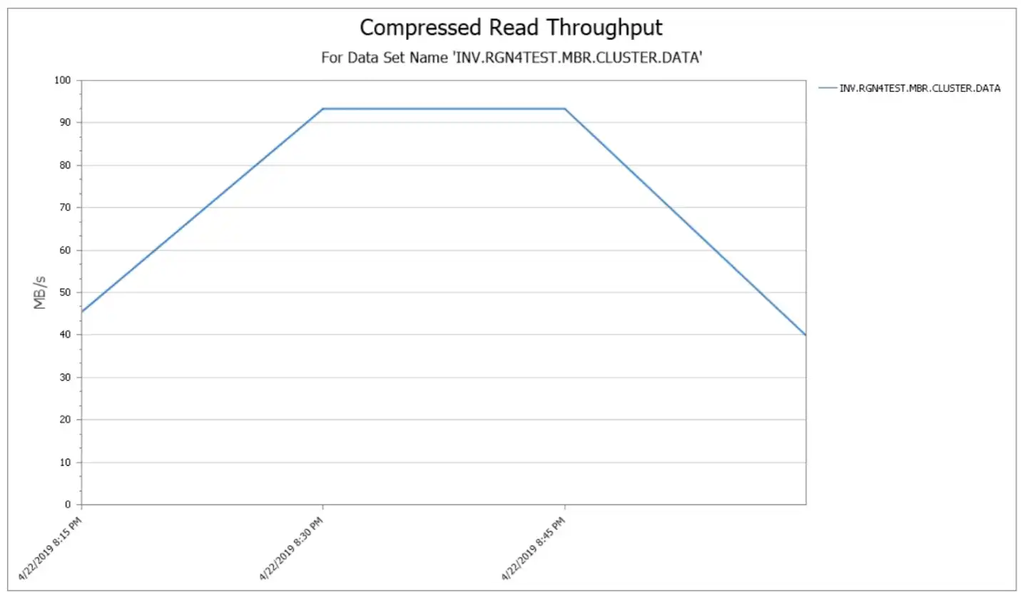
Figure 3: Compressed Read Throughput by time
Dataset Encryption
Dataset encryption is another optional feature of Extended Format datasets. File or data set encryption provides broad coverage for sensitive data by using encryption that is tied to access control for in-flight and at-rest data protection that is enabled by policy. Data is encrypted in bulk with low overhead by using the IBM Z integrated cryptographic hardware.
z/OS data set encryption supports extended-format sequential and VSAM datasets that can then also be used by z/OS zFS, IBM Db2, IBM IMS, middleware, logs, batch, and Independent Software Vendor (ISV) solutions.
Applications or middleware that use extended-format data that is accessed with VSAM, QSAM, or BSAM access methods can also use z/OS data set encryption.
When Db2 uses z/OS dataset level encryption, data in the Db2 or IMS buffer pools is not encrypted. IBM Security Guardium® Data Encryption for z/OS provides that extra level of security. This feature is an optional software feature that provides encryption at the Db2 row level and IMS segment level, and also encryption of data in memory and data in storage for Db2 and IMS. This feature can be layered on top of z/OS data set encryption when memory buffers must be encrypted. For more information about IBM Guardium Data Encryption for z/OS, see the IBM Guardium Data Encryption for Db2 and IMS Databases website.
Use SMF 42 Records for Deeper Understanding of Datasets
Oftentimes it is sufficient to analyze I/O performance analysis at the volume level of storage without needing to understand the datasets that comprise the volume or without understanding the applications that use those datasets. The SMF 42 records are useful to obtain a deeper understanding of the datasets and the applications that are using the storage. IntelliMagic Vision provides useful reports based on these statistics.
Besides identifying the dataset names, SMF 42 identifies the job name (in the case of batch jobs) or the address space name (in the case of a database subsystem such as Db2). It includes the WLM Service Class name and Workload name. SMF 42 also describes the type of dataset (e.g. physical sequential, extended format, linear….), the block size or CI size, the number of DFSMS stripes, the volsers of each dataset component, the type of compression or encryption, and the SMS Storage Class name. If the dataset is a VSAM dataset, SMF 42 indicates the type of access method (NSR, LSR, GSR or RLS).
To learn more about IntelliMagic Vision’s support for Db2, please visit: intellimagic.com/db2
Discover Modern Db2 Performance Monitoring
Learn how to add predictive and prescriptive value to your Db2 and CICS monitoring process with new analytics capabilities.
This article's author
 Jeff Berger
 Related Resources
What's New with IntelliMagic Vision for z/OS? 2024.1
January 29, 2024 | This month we've introduced updates to the Subsystem Topology Viewer, new Long-term MSU/MIPS Reporting, updates to ZPARM settings and Average Line Configurations, as well as updates to TCP/IP Communications reports.
What's New with IntelliMagic Vision for z/OS? 2024.2
February 26, 2024 | This month we've introduced changes to the presentation of Db2, CICS, and MQ variables from rates to counts, updates to Key Processor Configuration, and the inclusion of new report sets for CICS Transaction Event Counts.
Top 10 IntelliMagic Vision Features Released in 2023
With over 160 announced product updates, 2023 was a spectacular year of releases for users of IntelliMagic Vision for z/OS. In this blog we try to narrow it down to the 10 most popular, helpful, and groundbreaking.
Book a Demo or Connect With an Expert
Discuss your technical or sales-related questions with our mainframe experts today