Part 1: Lower MLC Software Costs with Processor Cache Optimization

It is common in today’s challenging business environments to find IT organizations intensely focused on expense reduction. For mainframe departments, this often leads to high priority expense reduction initiatives for IBM Monthly License Charge (MLC) software, which is typically the single largest line item in their budget.

IBM recently introduced a software pricing option that changes the basis of pricing, replacing the monthly peak four hour rolling average (4HRA) with charging for all CPU usage for the entire month (at a significantly reduced unit price). This new pricing model is called the Enterprise Consumption (EC) solution within Tailored Fit Pricing (TFP). Unit pricing for EC is customer-specific and derived from a baseline of your software expense from the prior 12 months, so sites considering a future migration to EC can achieve perpetual benefit from optimizing their savings within their current monthly peak 4HRA-based model prior to the migration.

The big differentiator is that since in an EC model all CPU generates software expense, the benefits of CPU reduction efforts extend to all work that runs at any time.

It is very important to realize that whether your site has already migrated to the EC model, you are planning for such a migration, or you anticipate remaining on a peak 4HRA-based model for the foreseeable future, in all of these scenarios reducing CPU consumption can translate into reduced software expense. The big differentiator is that since in an EC model all CPU generates software expense, the benefits of CPU reduction efforts extend to all work that runs at any time. This is in contrast to sites operating in a peak 4HRA-based model, where benefit is only realized when efficiencies are identified for workloads executing during the monthly peak interval.

This article begins a four-part series focusing on an area that has the potential to produce significant CPU savings, namely processor cache optimization. The magnitude of the potential opportunity to reduce CPU consumption and thus MLC expense available through optimizing processor cache is unlikely to be realized unless you understand the underlying concepts and have clear visibility into the key metrics in your environment.

Subsequent articles in the series will focus on ways to improve cache efficiency, through optimizing LPAR weights and processor configurations, and on improvements you can expect in this area from enhancements in the architecture of recent IBM processor models. Insights into the potential impact of various tuning actions will be illustrated with data from numerous real-life case studies, gleaned from experience gained from analyzing detailed processor cache data from 70 sites across 8 countries.

The role played by processor cache utilization became much more prominent with the significant change in hardware manufacturing technology that began with the z13 processor.[1] Achieving the rated capacity increases on z13 and subsequent models despite minimal improvements in machine cycle speeds is very dependent on effective utilization of processor cache. This article will begin by introducing key processor cache concepts and metrics that are essential for understanding the vital role processor cache plays in CPU consumption.

Key Metric: Cycles per Instruction

Cycles per instruction (CPI) and its components are key metrics for optimizing processor cache. CPI represents the average number of processor cycles spent per completed instruction. Conceptually, processor cycles are spent either productively, executing instructions and referencing data present in Level 1 (L1) cache, or unproductively, waiting to stage data due to L1 cache misses.^[2] Keeping the processor productively busy executing instructions is highly dependent on effective utilization of processor cache.

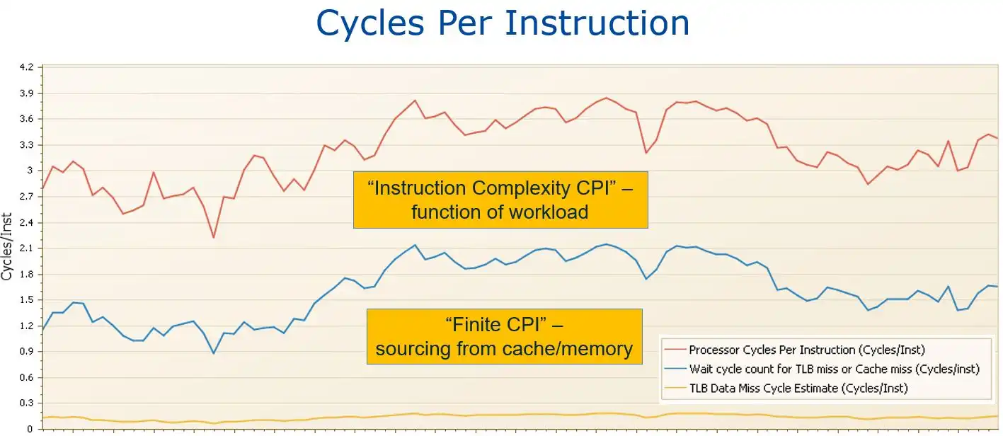
Figure 1: Cycles per instruction (CPI).

Figure 1 breaks out CPI into the “productive” and “unproductive” components just referenced.^[3] The space above the blue and below the red line reflects the cycles productively spent executing instructions for a workload. This would be the CPI value if all required data and instructions were always present in L1 cache, and is called “Instruction Complexity CPI” because it reflects the mix of simple and complex machine instructions in a business workload.

But since in reality there is a finite amount of L1 cache, limited to a size that can be accessed in a single machine cycle, machine cycles spent waiting for data and instructions to be staged from processor cache or memory into L1 cache are quantified as “Finite CPI”. Note that these waiting cycles, represented by the area under the blue line in Figure 1, represent a significant portion of the total, typically 30-50% of total CPI.

This sizable contribution of “waiting on cache” cycles toward overall CPU consumption on today’s z processors represents one of the primary takeaways of this entire series of articles. It highlights the magnitude of the potential opportunity if improvements in processor cache efficiency can be achieved and the importance of having clear visibility into key cache metrics in order to identify any such opportunities.

HiperDispatch

A key technology to understand when seeking to reduce those waiting cycles (Finite CPI) is HiperDispatch (HD). HD was first introduced in 2008 with z10 processors, but it plays an even more vital role on z13 and subsequent models where cache performance has such a big impact.

HD involves a partnership between the z/OS and PR/SM dispatchers to establish affinities between units of work and logical CPs, and between logical and physical CPs. This is important because it increases the likelihood of units of work being re-dispatched back on the same logical CP and executing on the same (or nearby) physical CP. This optimizes the effectiveness of processor cache at every level by reducing the frequency of processor cache misses, and by reducing the distance into the shared processor cache and memory hierarchy (called the nest) required to fetch data. This latter “distance” factor is very important because access time increases significantly for each subsequent level of cache and thus results in more waiting by the processor [Kyne2017].

When HD is active, PR/SM assigns logical CPs as Vertical Highs (VH), Vertical Mediums (VM), or Vertical Lows (VL) based on LPAR weights and the number of physical CPs. VH logical CPs have a one-to-one relationship with a physical CP. VMs have at least a 50% share of a physical CP. VLs have no guaranteed share, they exist to exploit unused capacity from other LPARs that are not using all of their share (and are subject to being “parked” when not in use).

Work executing on VHs optimizes cache effectiveness because its one-to-one relationship with a physical CP means it will consistently access the same processor cache. On the other hand, VMs and VLs may be dispatched on various physical CPs where they will be contending for processor cache with workloads from other LPARs, making the likelihood of their finding the data they need in cache significantly lower.

This intuitive understanding of the benefit of maximizing work executing on VHs is confirmed by multiple data sources. One such source is calculated estimates of the life of data in various levels of processor cache (derived from SMF 113 data). Commonly, cache working set data remains in L1 cache for less than 0.1 millisecond (ms), in L2 cache for less than 2 ms, and in L3 cache around 10 ms. This means that by the time an LPAR gets re-dispatched on a CP after another LPAR executed there for a typical PR/SM time-slice of 12.5 ms, its data in L1, L2 and L3 caches will all be gone. The good news is those working sets will be rebuilt quickly from L4 cache, but the bad news is that each access to L4 cache may take hundreds of cycles.

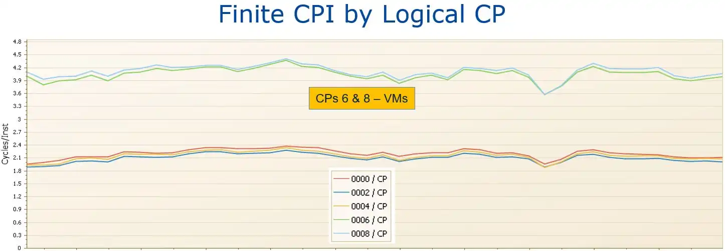
Figure 2: Finite CPI by Logical CP Sys18 (3 VHs,2 VMs).

This thesis that work executing on VHs experiences better cache performance is further substantiated by analyzing Finite CPI data at the logical CP level. At the beginning of the case study presented in Figure 2, the Vertical CP configuration for this system consisted of three VHs and two VMs. Note that the Finite CPI values for the two VM logical CPs (CPs 6 and 8) on this system were significantly higher than those for the VHs.[4]

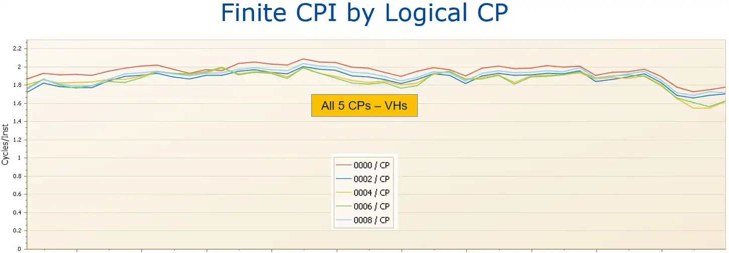
Figure 3: Finite CPI by Logical CP Sys18 (5 VHs).

Following the deployment of additional hardware that caused the Vertical CP configuration to change to five VHs (Figure 3), all the logical CPs had very similar Finite CPI values. In particular, now that CPs 6 and 8 were no longer VMs and were no longer experiencing cross-LPAR contention for processor cache, their “waiting on cache” cycles decreased to a level comparable to the other VHs.

Recap

Up to this point we have seen that CPI decreases when there is a reduction in unproductive machine cycles waiting for data and instructions to be staged into L1 cache. Reducing CPI translates directly to decreased CPU consumption, which as identified in the introduction translates into reduced IBM MLC software expense under any licensing scenario.

Opportunities to optimize processor cache are worth investigating because those unproductive waiting cycles typically represent at least one third to one half of overall CPU. Fortunately, the mainframe is a very metric rich environment, and metrics like Finite CPI are available that quantify those unproductive waiting cycles.

Some environments have achieved major CPU reductions through optimizing processor cache, others have identified smaller gains, and in some sites such opportunities may be minimal. There are no “silver bullets”, no single solution that will benefit every site. But understanding cache concepts and having good visibility into the metrics positions you to identify any opportunities that may exist in your environment. In the next article in the series we will begin exploring configuration changes and approaches others have used to reduce CPU driven by waiting on cache cycles.

Read Part 2: How Optimizing LPAR Configurations Can Reduce Software Expense

Sources

[Kyne2017] Frank Kyne, Todd Havekost, and David Hutton, CPU MF Part 2 – Concepts, Cheryl Watson’s Tuning Letter 2017 No. 1.

[1] This change from multi-chip modules (MCMs) to single-chip modules (SCMs), which reduced manufacturing costs and power consumption, introduced a non-uniform memory access (NUMA) topology which brought about more variability in latency times for cache accesses.

[2] While “waiting to stage data” z processors leverage Out of Order execution and other types of pipeline optimizations behind the scenes seeking to minimize unproductive waiting.

[3] A small subcomponent of Finite CPI, Translation Lookaside Buffer (TLB) misses while performing Dynamic Address Translation, is represented by the yellow line on Figure 1.

[4] The atypical magnitude of the gap on this system, which we might call the “VM penalty”, was impacted by adverse LPAR topology, which will be explored in the next article in this series.